How to Do a VLOOKUP in an Excel Spreadsheet

VLOOKUP won’t be as intuitive as different capabilities, but it surely’s a robust device price studying. Check out some examples and learn to use VLOOKUP on your personal Excel tasks.

What Is VLOOKUP in Excel?

Excel’s VLOOKUP perform is much like a phone e book. You present it with a worth to search for (like somebody’s title), and it returns your chosen worth (like their quantity).

VLOOKUP may appear daunting at first, however with a number of examples and experiments, you will quickly be utilizing it with out breaking a sweat.

The syntax for VLOOKUP is:

        =VLOOKUP(lookup_value, table_array, col_index_num[, exact])
    

This spreadsheet incorporates pattern knowledge to point out how VLOOKUP applies to a set of rows and columns:

On this instance, the VLOOKUP system is:

        =VLOOKUP(I3, A2:E26, 2)
    

Let’s have a look at what every of those parameters means:

• lookup_value is the worth that you just need to search for within the desk. On this instance, it is the worth in I3, which is 4.
• table_array is the vary that incorporates the desk. Within the instance, that is A2:E26.
• col_index_no is the column variety of the returned desired worth. The colour is within the second column of table_array, so that is 2.
• actual is an non-compulsory parameter figuring out whether or not the lookup match ought to be actual (FALSE) or approximate (TRUE, the default).

You should utilize VLOOKUP to show the returned worth or mix it with different capabilities to make use of the returned worth in additional calculations.

The V in VLOOKUP stands for vertical, which means that it searches a column of knowledge. VLOOKUP solely returns knowledge from columns to the correct of the lookup worth. Regardless of being restricted to the vertical orientation, VLOOKUP is a necessary device that makes different Excel duties simpler. VLOOKUP can turn out to be useful whenever you’re calculating your GPA and even evaluating two columns.

The right way to Do a VLOOKUP in Excel

Now that you understand how Excel’s VLOOKUP works, utilizing it’s only a matter of selecting the best arguments. If you happen to discover typing the arguments troublesome, you can begin the system by typing in an equal signal (=) adopted by VLOOKUP. Then click on the cells so as to add them as arguments within the system.

Let’s follow on the pattern spreadsheet above. Assume you might have a spreadsheet containing the next columns: Title of merchandise, Opinions, and Value. You then need Excel to return the variety of opinions for a specific product, Pizza on this instance.

You may simply obtain this with the VLOOKUP perform. Simply bear in mind what every argument will probably be. On this instance, since we need to search for details about the worth in cell E6, E6 is the lookup_value. The table_array is the vary containing the desk, which is A2:C9. You must solely embrace the info itself, with out the headers within the first row.

Lastly, the col_index_no is the column within the desk the place the opinions are, which is the second column. With these out of the best way, let’s get to writing that system.

1. Choose a cell the place you need to show the outcomes. We’ll go together with F6 on this instance.
2. Within the system bar, sort =VLOOKUP(.

   

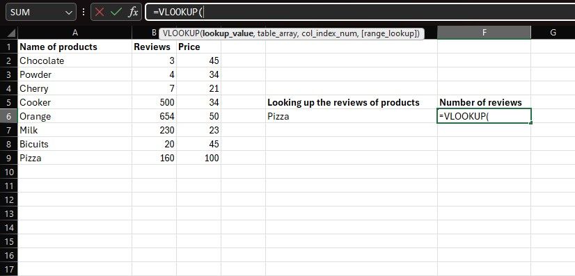
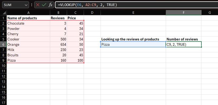
3. Spotlight the cell containing the lookup worth. That’s E6 on this instance, which incorporates Pizza.
4. Kind a comma (,) and an area, after which spotlight the desk array. That’s A2:C9 on this instance.
5. Subsequent, sort within the column variety of the specified worth. The opinions are within the second column, in order that’s 2 for this instance.
6. For the final argument, sort FALSE if you need an actual match of the merchandise you entered. In any other case, sort TRUE to see the closest match for it.

   

7. Finish the system with a closing parenthesis. Keep in mind to place a comma between the arguments. Your ultimate system ought to seem like under:

           =VLOOKUP(E6,A2:C9,2,FALSE)
       

8. Hit Enter to get your consequence.

   

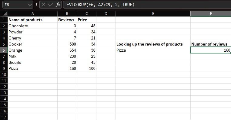
Excel will now return the opinions for Pizza in cell F6.

The right way to Do a VLOOKUP for A number of Objects in Excel

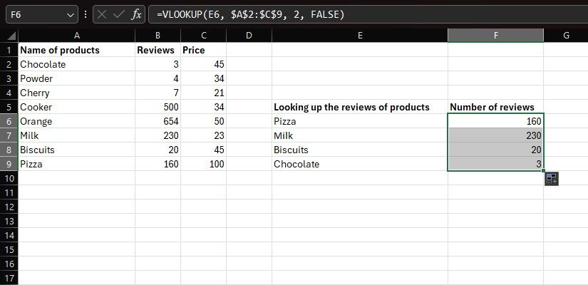
You can even search for a number of values in a column with VLOOKUP. This could turn out to be useful when it is advisable carry out operations like plotting Excel graphs or charts on the ensuing knowledge. You are able to do this by writing the VLOOKUP system for the primary merchandise after which auto-filling the remaining.

The trick is to make use of absolute cell references so they do not change throughout autofill. Let’s have a look at how you are able to do this:

1. Choose the cell subsequent to the primary merchandise. That is F6 on this instance.
2. Kind the VLOOKUP system for the primary merchandise.
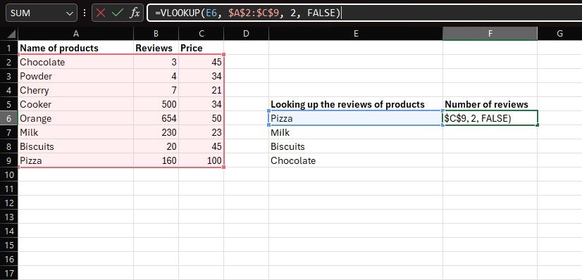
3. Transfer your cursor to the desk array argument within the system and press F4 in your keyboard to make it an absolute reference.

   

4. Your ultimate system ought to seem like under:

           =VLOOKUP(E6,$A$2:$C$9,2,FALSE)
       

5. Press Enter to get the outcomes.
6. As soon as the consequence seems, drag the outcomes cell right down to fill the system in for all the opposite objects.

   

The right way to Join Excel Sheets With VLOOKUP

You can even draw data from one Excel sheet to a different utilizing VLOOKUP. That is notably helpful if you wish to depart the unique desk unaffected, like whenever you’ve imported the info from an internet site to Excel.

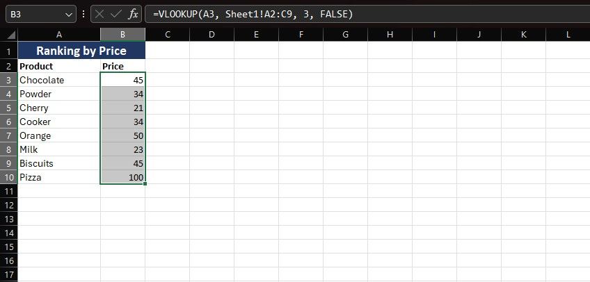
Think about that you’ve a second spreadsheet the place you need to type the merchandise from the earlier instance based mostly on their worth. You may get the value for these merchandise from the father or mother spreadsheet with VLOOKUP. The distinction right here is that you will have to go to the father or mother sheet to pick the desk array. Here is how:

1. Choose the cell the place you need to show the value of the primary merchandise. That is B3 on this instance.
2. Kind =VLOOKUP( within the system bar to start out the system.

   

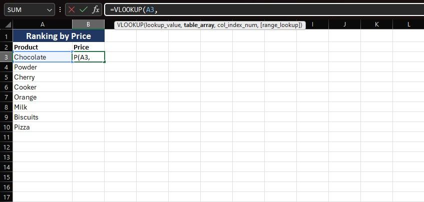
3. Click on the cell containing the primary merchandise’s title to append it because the look-up worth. That is A3 (Chocolate) on this instance.
4. Like earlier than, sort a comma (,) and an area to maneuver to the subsequent argument.
5. Navigate to the father or mother sheet and choose the desk array.

   

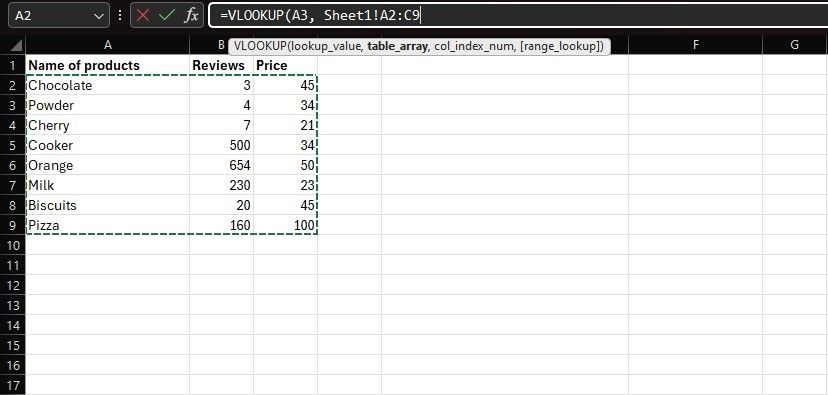
6. Hit F4 to make the reference absolute. This makes the system relevant to the remainder of the objects.
7. Whereas nonetheless on the father or mother sheet, have a look at the system bar and sort the column quantity for the value column. That is 3 on this instance.
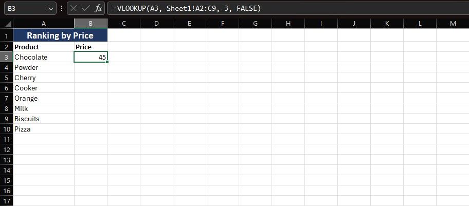
8. Kind FALSE because you need an actual match of every product on this case.

   

9. Shut the parenthesis and hit Enter. The ultimate system ought to seem like under:

           =VLOOKUP(A3, Sheet1!$A$2:$C$9, 3, FALSE)
       

10. Drag down the consequence for the primary product to see outcomes for the opposite merchandise within the subset sheet.

    

Now you can type your Excel knowledge with out it affecting the unique desk. Typos are one of many widespread causes of VLOOKUP errors in Excel, so be sure to keep away from them within the new checklist.

VLOOKUP is a good way to question knowledge quicker in Microsoft Excel. Though VLOOKUP solely queries inside a column and has a number of extra limitations, Excel has different capabilities that may do extra highly effective lookups.

Excel’s XLOOKUP perform is much like VLOOKUP however can look each vertically and horizontally in a spreadsheet. Most of Excel’s lookup options comply with the identical course of, with only some variations. Utilizing any of them for any particular lookup objective is a great strategy to come up with your Excel queries.